Statistics

A person who doesn't stop to consider the assumptions of the techniques she's using is, in effect, thinking that her techniques are magical

Overview

Approaches

Descriptive Statistics

a summary of data that quantitatively describes or summarizes features from a collection of information
aim is to summarize a sample
- It is therefore parametric
  - ie. the analysis of the statistical set is based on parameters, like variance, or a central tendency (ie. mean, median, mode, range)
    - a central tendency is often contrasted with its own level of variance
    - both central tendencies and their levels of variance are considered main properties of a distribution. With them we may judge whether a set of data has a strong central tendency based on the level of variance that it has.
ex. mean, standard deviation
spec: description statistics are backward looking, inductive statistics are forward looking
descriptive statistics does not rest on the assumption that the data came from a larger population

Inferential (Inductive) Statistics

aim is to learn about the population that the sample represents
- Therefore, it is developed on the basis of probability theory and by definition, cannot be parametric
Statistical inference is the process of analyzing data to make inferences on an underlying
Descriptive stats do add valuable context when trying to analyze data inductively.
- ex. in papers reporting on human subjects, typically a table is included giving the overall sample size, sample sizes in important subgroups, as well as demographic info like age, sex, ethnicity
The conclusion of a statistical inference is called a statistical proposition

Probability Distribution

def - the mathematical function that tells us the probability that each possible outcome occurs.
It is a mathematical representation of a random phenomenon
It is a function which takes the sample space (ie. all possible outcomes) as an input, and returns us the probability of their occurrence.
- ex. of a coin flip, sample space = {HEADS, TAILS}
- In other words, we give the function a single possible outcome, and the graph gives us the probability of that outcome occurring (the outcome of an event occurring is a subset of the sample space.
the probability distribution and the random variables which they describe underlies the mathematical discipline of probability theory
Probability distributions are more preferable than simple numbers for describing a quantity because:
1. There is spread or variability in almost any value that can be measured in a population
2. almost all measurements are made with some intrinsic error
  - ex. in physics many processes are described probabilistically
Common probability distributions:
- normal distribution, which is related to linear growth
- pareto distribution (pareto principle), which is related to exponential growth

Discrete Probability Distribution

All binomial distributions are discrete
- in other words, they are composed of discrete random variables
  - variable here, refers to the potential outcomes (observations) that can occur
The set of possible outcomes is discrete and predictable
- ex. coin toss, dice roll

Continuous Probability Distribution

All normal distribtions are continuous
The set of possible outcomes can take place on a continuous range
- ex. temperatures
These probabilities are described by a probability density function (PDF)
- This function takes in a single sample from the sample space and returns us "the probability that the input variable would equal that sample in real life"
- ex. what is the probability that the temperature at 7:00PM, as measured in reality, is equal to the sample recorded in this sample?
the absolute likelihood for a continuous random variable to take on any particular value is 0
- This is because there are an infinite set of possible values (ie. infinite sample space)

Univariate/Multivariate Distribution

Univariate - The probability distribution of only 1 random variable
Multivariate - The probability distribution of multiple random variables (a vector)
- regression towards the mean can be defined for any bivariate distribution with identical marginal distributions

Kurtosis

a staple of probability theory
It is a measure of dispersion (along with variance, skewness and min/max values)

Kurtosis is a measure of the "tailedness" of a distribution

- In other words, the sharpness of the peak of the bell curve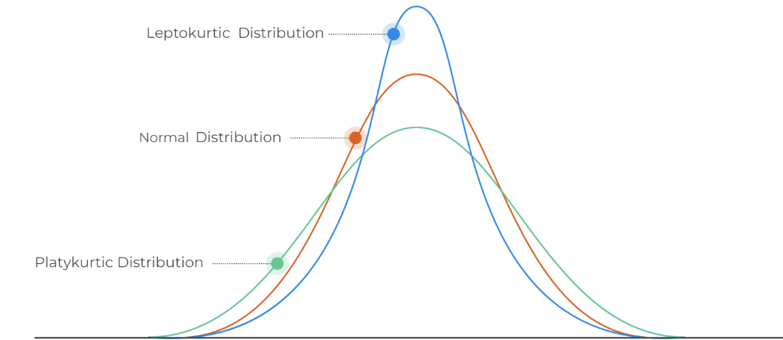

The first step when analyzing any statistical analysis is what ways are they measuring the parameters. For instance if we are measuring popularity of websites have a certain date range, then we would have to know are you calculating that by how many visits the sites gets or are you talking about how much time is spent on each site, and so on by asking questions like this we understand better the true intentions of the author of the analysis

The way the overall proportion of coin flips settles down to 50% isn’t that fate favors tails to compensate for the heads that have already landed; it’s that those first ten flips become less and less important the more flips we make.

The null hypothesis, in executive bullet-point form:

Run an experiment.
Suppose the null hypothesis is true, and let p be the probability (under that hypothesis) of getting results as extreme as those observed.
The number p is called the p-value.
If it is very small, rejoice; you get to say your results are statistically significant.
If it is large, concede that the null hypothesis has not been ruled out.

“Statistically noticeable” or “statistically detectable” would be a better term than “statistically significant”

That would be truer to the meaning of the method, which merely counsels us about the existence of an effect but is silent about its size or importance.

The purpose of statistics isn’t to tell us what to believe, but to tell us what to do. Statistics is about making decisions, not answering questions.

Pie charts should not have more than 3 variables included

reasoning: when there are more than 3, our eyes start playing tricks and we are no longer able to draw conclusions from the visualization
- verify this claim (originally from Layton)

Faking randomness

When people try to purposely make something look random, it ends up being evidence that it wasn't a random process at all. Chunks occur naturally in a randomized process. When we try to fake it, we naturally avoid chunking. This is a clue that it was a faked process.
ex. 7738499 is more likely to be a random number than 3950681. the second example has no chunked numbers, and no repeated numbers. This looks deliberately crafted to seem random.

Population vs Sample

population denotes all members of a group.
- spec: Depending on what we are looking at, and what we are interested in, within the stock market, a populate could be every single stock in existence, or it could be every stock in the S&P500.
- populations are difficult to observe in real life
  - ex. how could we realistically obtain the data with every single student at a university included?
sample denotes that we are taking some subset of this population for analysis purposes
The goal of statistics is to gather and analyze data from a sample, that also serves as a good representation of the entire population
a good sample: each unit in the sample should have had equal % opportunity to enter the sample (from the population).
- ex. if we wanted to get a sample of all students, and went and chose 50 people in the Gym, we are getting a bad sample, because the likelihood of any one person in the gym getting selected for the sample is higher than the likelihood of any one person in the library getting selected for the sample. We are not getting a good representation of the population
Samples should be both 100% (ideally) random and representative of the population
Statistics are derived from samples, while Parameters are derived from populations
- At a particular time, there may exist a Parameter for the percentage of all voters in USA who prefer Donald Trump, but we obviously can't ask everyone, so we need to take a sample.
- Parameters are therefore more of an ephemeral value that can't actually be obtained in the current moment. We use samples to try and get as close to that parameter as we can.

Variance, Standard Deviation, Coefficient of Variation

Variance

measures how far a set of numbers are spread out from their average value
- a measure of dispersion of a datapoint around its mean
each data point will be a certain distance away from the mean line. This is the variance of a given period
variance = sum of squared differences between observed values (the points on a plot) and the population mean (the straight line), divided by total # of observations
- in other words, variance is a function of how far those observed values are from the mean line
Mathematically, the variance of the sample = variance of the population / sample size
- This is because as the sample size increases, sample means cluster more closely around the population mean.

Standard Deviation (σ)

equal to square root of Variance
SD is more useful than variance, and variance's biggest value is in letting us easily calculate SD
SD is closer to the reality of what it is we are sampling.
- ex. we have a sample of 10 stock prices and have calculated the SD=3. Since the units we used for the calculation was $1, the SD is also in terms of $1 (ie. SD is $3)
unable to compare different datasets with SD alone (need CV)

Covariance (cov)

the relationship between two variables
- ex. stock price
covariance is not the same thing as correlation, but covariance is used in the formula to determine correlation
a higher covariance means the stocks tend to move together. Negative covariance means they have little correlation.
- verify this. I suspect that negative value means "negative correlation", not "no correlation". This would make 0 "not correlated at all"
like variance, covariance is not a standardized value
- To get a more comparable value, we will need to convert to correlation
Modern Portfolio Theorists believe that the key is to build a portfolio composed of stocks that have low covariance.
- It is a way to remove non-systemic risk

Standard error (SE)

def - the SD between samples of a single population
- spec: Therefore, we are getting an idea of how well we sampled the data. The more random and representative a piece of data is, the better sample it is. Therefore, if we got another sample from the same population and there was no variance, we would know we did a perfect job of getting a sample.
usually "Standard Error" refers to "Standard Error of the Mean" (ie. we are measuring the "mean" statistic)
standard deviation is commonly used to measure confidence in statistical conclusions
- ex. margin of error determined by calculating the expected standard deviation

Use

With a statistical observation (plotted on a graph), we would have applied formulas to make observations. When we know the SE, we are able to recalculate those formulas with the added benefit of having the SE. This effectively allows us to incorporate the effect of the SE into the function that we have used to generate (secondary) data.

Coefficient of Variation (CV)

equal to SD / mean
It simply exists to standardize the variation of a distribution.
With this number, we can compare the SD of different datasets
- ex. we are looking at a restaurant menu with prices in both USD and CAD. Ultimately, The SD of each dataset will be different, but the CV will be identical between the datasets
tells us the SD relative to the mean
pitfalls

Distributions

Normal Distribution

A normal distribution of data is like rolling a pair of dice. We know that over many rolls, the most common result from the dice will be seven, and the least common results will be two and twelve.

It is a characteristic of normal distributions that 1SD from the mean will cover 68% of cases, 2SD will cover 96% of cases, and 3SD will cover 99.9% of cases.

Central Limit Theorem

as the sample size gets larger, the sampling distribution of the mean approaches a normal distribution
theorem holds especially true for samples sizes over 30
ex. if we take 2 die and roll them 1000 times, we will find that the each observed sum will form in the shape of a bell curve, with 7 being in the center and 14 and 2 being in the tails.

Fat Tail Curves

if we take A bell curve, we know that the extremes are predictable. we have a tough percentage probabilities that an event in the tail will come to pass. however, with fat tail, we have a situation where there are many unlikely extreme events. each event is still equally as unlikely, but there are a lot more of them, making an extreme outcome more likely than with a bell curve

the more extreme events that are possible, the higher the probability that one of them will occur
explanation: think of a the heights of a population (normal distribution). there are outliers, but there is a cap on how extreme they will be. we will not see a man 10x the height of the average. but with a curve with fat tails, like wealth, we regularly meet people who are 1000s of times wealithier than the average
its a logical fallacy to compare statistics of normal distributions and fat tails
ex. there are twice as many deaths from slipping and falling on your head than there are from terrorist attacks. therefore we shouldn't be concerned. the problem with this statement is that slipping and falling is normal distribution, while terrorist attacks are fat tail. put another way, deaths from falling down stairs is pretty bounded. there wont be a 10x increase all of a sudden. the same cant be guaranteed for terrorist attacks
Fat tail is just a technical term for Black Swan Events

Marginal Distribution

def - the probability distribution of the variables contained in a subset of data

- ex. given a sample of 100 students and their relation between the amount of time they study and their resulting grades, we can plot what these numbers look like. This is the marginal distribution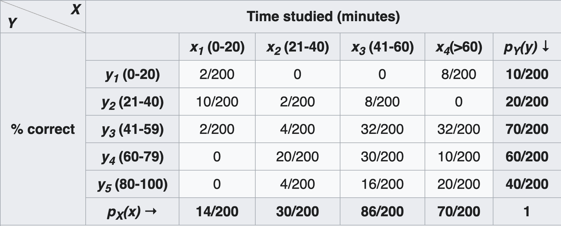

- by adding up the values in the top row (8/200 + 2/100), we can easily determine that 5% of students get a grade of <= 20%

Once we have this, we can use conditional distribution to answer questions like: "what is the probability a student studied for 10 hours and received a grade of 20% or less?"
ex. Imagine we are trying to determine the odds of getting hit by a car while crossing the street with a traffic light (at various colors). We will define 2 discrete random variables:
1. H={hit,not hit}
2. L={red,yellow,green}
- H depends on L. In other words, your likelihood of getting hit are increased if L=green.
- This means that for any given pair of H and L, we must consider the bivariate (joint) probability distribution of H and L. We need to determine the probability of that particular pair of events occurring if the pedestrian ignores the state of the light.
- In trying to figure out the marginal probability of being hit P(H=hit), what we are interested in is the probability that the pedestrian is hit, where the color of the light is unknown, and the pedestrian ignores the color of the light
- In this example, we need to know the duration of time each light is on (ie. the probability of any one light being on), and we need to know the probability of getting hit by a car, given the color of the light

Why we square the differences

This serves 2 main purposes

1. Gives us a positive number
	- We square in situations where we are looking for *magnitude*, and don't care about the direction of that magnitude (ex. variance)
	- Also if we just add up the first numbers without squaring, we will net out at zero 
2. Amplifies the effect of large differences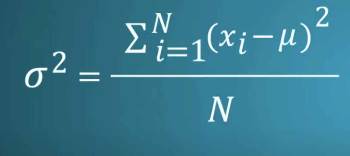

Law of large numbers

As individuals, people are completely unpredictable. Okay? One person making one bet... I couldn't possibly tell you what they're going to do. But the law of large numbers tells me that a million people making a million bets? That is completely predictable. Completely ordered.

Pitfalls with statistics

Non-linear correlation

Pearson's Correlation Coefficient only considers a linear relationship. for instance, if we are measuring the relationship between vitamin intake and health, it will be correlated to an extent, then will level off. applying pearsons correlation coefficient here will show the two as being only tenuously correlated
- related

Type I & Type II Errors

Equivalent to False Positive (type I) and False Negative (type II)
These are the two kinds of errors in a binary test
Intuitively, type I errors can be thought of as errors of commission, and type II errors as errors of omission
- ex. if we are shown a blurry picture and asked to identify it, an error of commission would be classifying the image as a dog, when it in fact isn't (type I). On the other hand, classifying the image as "not a dog", when it in fact is, would be an error of omission.

Confidence Interval

if a confidence level is 90%, that means that in 90% of the samples taken (from a larger population), the interval estimate will contain the population parameter confidence levels are determined before any analysis (so we don't make the analysis fit the data). 95% confidence level is most common

Factors affecting the width of the confidence interval include the size of the sample, the confidence level, and the variability in the sample interpreting
"Were this procedure to be repeated on numerous samples, the fraction of calculated confidence intervals (which would differ for each sample) that encompass the true population parameter would tend toward 90%."
The confidence interval can be expressed in terms of a single sample: "There is a 90% probability that the calculated confidence interval from some future experiment encompasses the true value of the population parameter."
The explanation of a confidence interval can amount to something like: "The confidence interval represents values for the population parameter for which the difference between the parameter and the observed estimate is not statistically significant at the 10% level" what it is not
A 95% confidence level does not mean that for a given realized interval there is a 95% probability that the population parameter lies within the interval (i.e., a 95% probability that the interval covers the population parameter). once an interval is calculated, this interval either covers the parameter value or it does not; it is no longer a matter of probability. The 95% probability relates to the reliability of the estimation procedure, not to a specific calculated interval

Correlation

relationships bind facts together, satisfying our human desire to have a narrative explain events (rather than acknowledge that randomness occurs)

Univariate analysis

univariate analysis is oversimplistic and fails to uncover the underlying reasons of why some phenomenon occurs ex. take the gender pay gap. It's indisputable that in the aggregate, men get paid 9% more than women. However, this oversimplification ignores important factors in pay. For instance, individuals with the personality trait known as Agreeableness tend to get paid less. Women on average tend to be more agreeable than men. Not all women are more agreeable than men, and those women on average get paid more. What if it were the case that a woman and a man have exactly the same personality, and they got paid the same? would that dispel the idea that there is a legitimate gap, or would it just further underline the individual reasons that result in that gender pay gap?

This underpins the issue with univariate analysis: you look at a single variable and attempt to understand the picture and all the reasons why that outcome has occurred. What you have failed to realize is that there may be 20 main factors that determine pay inequality, and gender and agreeableness might only constitute 2 of them.
Other underlying differences between women and men that may help explain the perceived pay gap: Women tend to be less inclined to take risks, armoire influenced by the chance of loss, or less competitive, and less status conscious.

Children

Backlinks

Intelligence